
For more information or if you need help retrieving your data, please contact Weights & Biases Customer Support at support@wandb.com
Although we’re only a few years removed from the transformer breakthrough, LLMs have already grown massively in performance, cost, and promise. At W&B, we’ve been fortunate to see more teams try to build LLMs than anyone else. But many of the critical details and key decision points are often passed down by word of mouth.
The goal of this white paper is to distill the best practices for training your own LLM for scratch. We’ll cover everything from scaling and hardware to dataset selection and model training, letting you know which tradeoffs to consider and flagging some potential pitfalls along the way. This is meant to be a fairly exhaustive look at the key steps and considerations you’ll make when training an LLM from scratch.
The first question you should ask yourself is whether training one from scratch is right for your organization. As such, we’ll start there:
Before you dive into training, it’s important to cover how LLMs scale. Understanding scaling lets you effectively balance the size and complexity of your model and the size of the data you’ll use to train it.
Some relevant history here: OpenAI originally introduced “the LLM scaling laws” in 2020. They suggested that increasing model size was more important than scaling data size. This held for about two years before DeepMind suggested almost the polar opposite: that previous models were significantly undertrained and that increasing your foundational training datasets actually leads to better performance.
That changed in 2022. Specifically, DeepMind put forward an alternative approach in their Training Compute-Optimal Large Language Models paper. They found that current LLMs are actually significantly undertrained. Put simply: these large models weren’t trained on nearly enough data.
Deepmind showcased this with a model called Chinchilla, which is a fourth the size of the Gopher model above but trained on 4.6x more data. At that reduced size but with far more training data, Chinchilla outperformed Gopher and other LLMs.
DeepMind claims that the model size and the number of training tokens* should instead increase at roughly the same rate to achieve optimal performance. If you get a 10x increase in compute, you should make your model 3.1x times bigger and the data you train over 3.1x bigger; if you get a 100x increase in compute, you should make your model 10x bigger and your data 10x bigger.
*Note: Tokenization in NLP is an essential step of separating a piece of text into smaller units called tokens. Tokens can be either words, characters, or subwords. The number of training tokens is the size of training data in token form after tokenization. We will dive into detailed tokenization methods a little later.
To the left of the minima on each curve, models are too small — a larger model trained on less data would be an improvement. To the right of the minima on each curve, models are too large — a smaller model trained on more data would be an improvement. The best models are at the minima.


DeepMind provides the following chart showing how much training data and compute you’d need to optimally train models of various sizes.

In summary, the current best practices in choosing the size of your LLM models are largely based on two rules:
It should come as no surprise that pre-training LLMs is a hardware-intensive effort. The following examples of current models are a good guide here:
• PaLM (540B, Google):
6144 TPU v4 chips used in total, made of two TPU v4 Pods connected over data center network (DCN) using a combination of model and data parallelism.
• OPT (175B, Meta AI):
992 80GB A100 GPUs, utilizing fully shared data parallelism with Megatron-LM tensor parallelism.
• GPT-NeoX (20B, EleutherAI):
96 40GB A100 GPUs in total.
• Megatron-Turing NLG (530B, NVIDIA & MSFT):
560 DGX A100 nodes, each cluster node has 8 NVIDIA 80-GB A100 GPUs.
Training LLMs is challenging from an infrastructure perspective for two big reasons. For starters, it is simply no longer possible to fit all the model parameters in the memory of even the largest GPU (e.g., NVIDIA 80GB-A100), so you’ll need some parallel architecture here. The other challenge is that a large number of compute operations can result in unrealistically long training times if you aren’t concurrently optimizing your algorithms, software, and hardware stack (e.g., training GPT-3 with 175B parameters would require about 288 years with a single V100 NVIDIA GPU).
Although we’re only a few years removed from the transformer breakthrough, LLMs have already grown massively in performance, cost, and promise. At W&B, we’ve been fortunate to see more teams try to build LLMs than anyone else. But many of the critical details and key decision points are often passed down by word of mouth.
The goal of this white paper is to distill the best practices for training your own LLM for scratch. We’ll cover everything from scaling and hardware to dataset selection and model training, letting you know which tradeoffs to consider and flagging some potential pitfalls along the way. This is meant to be a fairly exhaustive look at the key steps and considerations you’ll make when training an LLM from scratch.
The first question you should ask yourself is whether training one from scratch is right for your organization. As such, we’ll start there:
Parallelization refers to splitting up tasks and distributing them across multiple processors or devices, such as GPUs, so that they can be completed simultaneously. This allows for more efficient use of compute resources and faster completion times compared to running on a single processor or device. Parallelized training across multiple GPUs is an effective way to reduce the overall time needed for the training process.
There are several different strategies that can be used to parallelize training, including gradient accumulation, micro-batching, data parallelization, tensor parallelization, pipeline parallelization, and more. Typical LLM pre-training employs a combination of these methods. Let’s define each:
Data parallelism is the best and most common approach for dealing with large datasets that cannot fit into a single machine in a deep learning workflow.
More specifically, data parallelism divides the training data into multiple shards (partitions) and distributes them to various nodes. Each node first works with its local data to train its submodel, and then communicates with the other nodes to combine their results at certain intervals in order to obtain the global model. The parameter updates for data parallelism can be either asynchronous or synchronous. The advantage of this method is that it increases compute efficiency and that it is relatively easy to implement. The biggest downside is that during the backward pass you have to pass the whole gradient to all other GPUs. It also replicates the model and optimizer across all workers which is rather memory inefficient.

Bad data leads to bad models. But careful processing of high-quality, high-volume, diverse datasets directly contributes to model performance in downstream tasks as well as model convergence.
Dataset diversity is especially important for LLMs. That’s because diversity improves the cross-domain knowledge of the model, as well as its downstream generalization capability. Training on diverse examples effectively broadens the ability of your LLM to perform well on myriad nuanced tasks.
A typical training dataset is comprised of textual data from diverse sources, such as crawled public data, online publication or book repositories, code data from GitHub, Wikipedia, news, social media conversations, etc.
For example, consider The Pile. The Pile is a popular text corpus created by EleutherAI for large-scale language modeling. It contains data from 22 data sources, coarsely broken down into five broad categories:
Note that The Pile dataset is one of the very few large-scale text datasets that is free for the public. For most of the existing models like GPT-3, PaLM, and Galactica, their training and evaluation datasets are not publicly available. Given the large-scale effort it takes to compile and pre-process these datasets for LLM training, most companies have kept them in-house to maintain a competitive advantage. That makes datasets like The Pile and a few datasets from AllenAI extremely valuable for public large-scale NLP research purposes.
Another thing worth mentioning is that, during dataset collection, general data can be collected by non-experts, but data for specific domains normally needs to be collected or consulted by subject matter experts (SMEs), e.g., doctors, physicists, lawyers, etc. SMEs can flag thematic or conceptual gaps that NLP engineers might miss. NLP engineers should also be heavily involved at this stage given their knowledge of how an LLM “learns to represent data” and thus their abilities to flag any data oddities or gaps in the data that SMEs might miss. Once you’ve identified the dataset(s) you’ll be using, you’ll want to prepare that data for your model. Let’s get into that now:
To ensure training data is high-quality and diverse, several pre-processing techniques can be used before the pre-training steps:
Certain data components can be up-sampled to obtain a more balanced data distribution. Some research down-samples lower-quality datasets such as unfiltered web crawl data. Other research up-samples data of a specific set of domains depending on the model objectives.
Due to its goals, the pre-training dataset is composed of high-quality data mainly from science resources such as papers, textbooks, lecture notes, encyclopedias. The dataset is also highly curated, for example, with task-specific datasets to facilitate the composition of this knowledge into new task contexts.
There are also advanced methods to filter high-quality data, such as using a trained classifier model applied to the dataset. For example, the model Galactica by Meta AI is built purposefully for science, specifically storing, combining, and reasoning about scientific knowledge.
To reduce the risk of training instabilities, practitioners often start with the model architecture and hyperparameters of a popular predecessor such as GPT-2 and GPT-3, making informed adjustments along the way to improve training efficiency, scale the size of the models (in both depth and width), and enhance performance. Two examples:
GPT-NeoX-20B (20B, EleutherAI) originally took GPT-3’s architecture and made these changes:
OPT-175B (175B, Meta AI) also built on GPT-3 and adjusted:
As we mentioned above, typical pre-training involves lots of experiments to find the optimal setup for model performance. Experiments can involve any or all of the following: weight initialization, positional embeddings, optimizer, activation, learning rate, weight decay, loss function, sequence length, number of layers, number of attention heads, number of parameters, dense vs. sparse layers, batch size, and dropout.
A combination of manual trial and error of those hyperparameter combinations and automatic hyperparameter optimization (HPO) are typically performed to find the optimal set of configurations to achieve optimal performance. Typical hyperparameters to perform automatic search on: learning rate, batch size, dropout, etc.
Hyperparameter search is an expensive process and is often too costly to perform at full scale for multi-billion parameter models. It’s common to choose hyperparameters based on a mixture of experiments at smaller scales and by interpolating parameters based on previously published work instead of from scratch.
In addition, there are some hyperparameters that need to be adjusted even during a training epoch to balance learning efficiency and training convergence. Some examples:

You’ll want to do a lot of this early in your pre-training process. This is largely because you’ll be dealing with smaller amounts of data, letting you perform more experiments early versus when they’ll be far more costly down the line.
Before we continue, it’s worth being clear about a reality here: you will likely run into issues when training LLMs. After all: these are big projects and, like anything sufficiently large and complicated, things can go wrong.
During the course of training, a significant number of hardware failures can occur in your compute clusters, which will require manual or automatic restarts. In manual restarts, a training run is paused, and a series of diagnostics tests are conducted to detect problematic nodes. Flagged nodes should then be cordoned off before you resume training from the last saved checkpoint.
Training stability is also a fundamental challenge. While training the model, you may notice that hyperparameters such as learning rate and weight initialization directly affect model stability. For example, when loss diverges, lowering the learning rate and restarting from an earlier checkpoint might allow the job to recover and continue training.
Additionally, the bigger the model is, the more difficult it is to avoid loss spikes during training. These spikes are likely to occur at highly irregular intervals, sometimes late into training.
There hasn’t been a lot of systematic analysis of principled strategies to mitigate spikes. Here are some best practices we have seen from the industry to effectively get models to converge:
Note: Most of the above model convergence best practices not only apply to transformer training but also apply in a broader deep learning context across architectures and use cases.
Finally, after your LLM training is completed, it is very important to ensure that your model training environment is saved and retained in that final state. That way, if you need to re-do anything or replicate something in the future, you can because you have the training state preserved.
A team could also try some ablation studies. This allows you to see how pulling parts of the model out might impact performance. Ablation studies can allow you to massively reduce the size of your model while still retaining most of a model’s predictive power.
Typically, pre-trained models are evaluated on diverse language model datasets to assess their ability to perform logical reasoning, translation, natural language inference, question answering, and more.
Machine learning practitioners have coalesced around a variety of standard evaluation benchmarks. A few popular examples include:

Another evaluation step is n-shot learning. This is a task-agnostic dimension and refers to the number of supervised samples (demonstrations) provided to the model right before asking it to perform a given task. N-shots are typically provided via a technique called prompting. These evaluations are often categorized into the following three groups:
Task: Sentiment Analysis
Prompt:
Tweet: “I hate it when my phone battery dies.”
Sentiment: Negative
Tweet: “My day has been amazing!”
Sentiment: Positive
Tweet: “This is the link to the article.”
Sentiment: Neutral
Tweet: “This new music video was incredible!”
Sentiment:
Answer: ______
Evaluation typically involves both looking at benchmarking metrics of the above tasks and more manual evaluation by feeding the model with prompts and looking at completions for human assessment. Typically, both NLP Engineers and subject matter experts (SMEs) are involved in the evaluation process and assess the model performance from different angles:
NLP engineers are people with a background in NLP, computational linguistics, prompt engineering, etc., who can probe and assess the model’s semantic and syntactic shortcomings and come up with model failure classes for continuous improvement. A failure class example would be: “the LLM does not handle arithmetic with either integers (1, 2, 3, etc.) nor their spelled-out forms: one, two, three.”
Subject matter experts (SMEs) are, in contrast to the NLP engineers, asked to probe specific classes of LLM output, fixing errors where necessary, and “talking aloud” while doing so. The SMEs are required to explain in a step-by-step fashion the reasoning and logic behind their correct answer versus the incorrect machine-produced answer.
There are potential risks associated with large-scale, general-purpose language models trained on web text. Which is to say: humans have biases, those biases make their way into data, and models that learn from that data can inherit those biases. In addition to perpetuating or exacerbating social stereotypes, you want to ensure your LLM doesn’t memorize and reveal private information.
It’s essential to analyze and document such potential undesirable associations and risks through transparency artifacts such as model cards.
Similar to performance benchmarks, a set of community-developed bias and toxicity benchmarks are available for assessing the potential harm of LLM models. Typical benchmarks include:
To date, most analysis on existing pre-trained models indicates that internet-trained models have internet-scale biases. In addition, pre-trained models generally have a high propensity to generate toxic language, even when provided with a relatively innocuous prompt, and adversarial prompts are trivial to find.
So how do we fix this? Here are a few ways to mitigate biases during and after the pre-training process:
Training set filtering: Here, you want to analyze the elements of your training dataset that show evidence of bias and simply remove them from the training data.
Training set modification: This technique doesn’t filter your training data but instead modifies it to reduce bias. This could involve changing certain gendered words (from policeman to policewoman or police officer, for example) to help mitigate bias.
Additionally, you can mitigate bias after pre-training as well:
Prompt engineering: The inputs to the model for each query are modified to steer the model away from bias (more on this later).
Fine-tuning: Take a trained model and retrain it to unlearn biased tendencies.
Output steering: Adding a filtering step to the inference procedure to re-weigh output values and steer the output away from biased responses.
At this point, let’s assume we have a pre-trained, general-purpose LLM. If we did our job well, our model can already be used for domain-specific tasks without tuning for few-shot learning and zero-shot learning scenarios. That said, zero-shot learning is in general much worse than its few-shot counterpart in plenty of tasks like reading comprehension, question answering, and natural language inference. One potential reason is that, without few-shot examples, it’s harder for models to perform well on prompts that are not similar to the format of the pretraining data.
To solve this issue, we can use instruction tuning. Instruction tuning is a state-of-the-art fine-tuning technique that fine-tunes pre-trained LLMs on a collection of tasks phrased as instructions. It enables pre-trained LLMs to respond better to instructions and reduces the need for few-shot examples at the prompting stage (i.e., drastically improves zero-shot performance).
Instruction tuning has gained huge popularity in 2022, given that the technique considerably improves model performance without hurting its ability to generalize. Typically, a pre-trained LLM is tuned on a set of language tasks and evaluated on its ability to perform another set of language tasks unseen at tuning time, proving its generalizability and zero-shot capability. See illustration below:

A few things to keep in mind about instruction tuning:
– Instruction tuning tunes full model parameters as opposed to freezing a part of them in parameter-efficient fine-tuning. That means it doesn’t bring with it the cost benefits that come with parameter-efficient fine-tuning. However, given that instruction tuning produces much more generalizable models compared to parameter-efficient fine-tuning, instruction-tuned models can still serve as a general-purpose model serving multiple downstream tasks. It often comes down to whether you have the instruction dataset available and the training budget to perform instruction tuning.
– Instruction tuning is universally effective on tasks naturally verbalized as instructions (e.g., NLI, QA, translation), but it is a little trickier for tasks like reasoning. To improve for these tasks, you’ll want to include chain-of-thought examples during tuning.


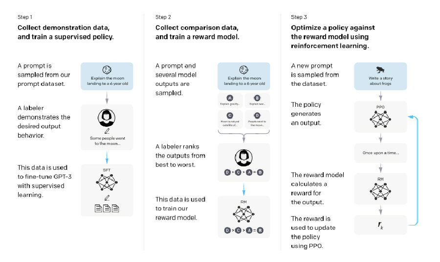
RLHF
RLHF (Reinforcement Learning with Human Feedback) extends instruction tuning by incorporating human feedback after the instruction tuning step to improve model alignment with user expectations.
Pre-trained LLMs often exhibit unintended behaviors, such as fabricating facts, generating biased or toxic responses, or failing to follow instructions due to the misalignment between their training objectives and user-focused objectives. RLHF addresses these issues by using human feedback to refine model outputs.
OpenAI’s InstructGPT and ChatGPT are examples of RLHF in action. InstructGPT, fine-tuned with RLHF on GPT-3, and ChatGPT, based on the GPT-3.5 series, demonstrate significant improvements in truthfulness and reductions in toxic outputs while incurring minimal performance regressions (referred to as the “alignment tax”).
Steps in RLHF:
Steps 2 and 3 are iterative, with new comparison data collected and used to refine the reward model and policy further.
Companies like Scale AI, Labelbox, Surge, and Label Studio offer RLHF as a service, facilitating its adoption without requiring in-house expertise. While RLHF can impose an alignment tax, research shows promising results in minimizing these costs, making it a viable approach for improving LLM performance.
To date, RLHF has shown very promising results with InstructGPT and ChatGPT, bringing improvements in truthfulness and reductions in toxic output generation while having minimal performance regressions compared to the pre-trained GPT.
Note that the RLHF procedure does come with the cost of slightly lower model performance in some downstream tasks—referred to as the alignment tax.
Companies like Scale AI, Labelbox, Surge, and Label Studio offer RLHF as a service, so you don’t have to handle this yourself if you’re interested in going down this path. Research has shown promising results using RLHF techniques to minimize the alignment cost and increase its adoption, making it absolutely worth considering.
Whether it’s OpenAI, Cohere, or open-source projects like EleutherAI, cutting-edge large language models are built on Weight & Biases. Our platform enables collaboration across teams performing the complex, expensive work required to train and push these models to production, logging key metrics, versioning datasets, enabling knowledge sharing, sweeping through hyperparameters, and a whole lot more. LLM training is complex and nuanced, and having a shared source of truth throughout the lifecycle of a model is vital for avoiding common pitfalls and understanding performance every step of the way.
We’d like to also send a hearty thanks to OpenAI, DeepMind, Meta, and Google Brain. We referenced their research and breakthroughs frequently in this white paper, and their contributions to the space are already invaluable.
If you’re interested in learning more about how W&B can help, please reach out and we’ll schedule some time. And if you have any feedback, we’d love to hear those too.


Since the advent of transformers, many architectural variants have been proposed. These can vary by architecture (e.g., decoder-only models, encoder-decoder models), by pretraining objectives (e.g., full language modeling, prefix language modeling, masked language modeling), and other factors.
While the original transformer included a separate encoder that processes input text and a decoder that generates target text (encoder-decoder models), the most popular LLMs like GPT-3, OPT, PaLM, and GPT-NeoX are causal decoder-only models trained to autoregressively predict a text sequence.
In contrast with this trend, there is some research showing that encoder-decoder models outperform decoder-only LLMs for transfer learning (i.e., where a pre-trained model is fine-tuned on a single downstream task). For detailed architecture types and comparison, see What Language Model Architecture and Pre-training Objective Work Best for Zero-Shot Generalization.
Here are a few of the most popular pre-training architectures:
Encoder-decoder models: As originally proposed, the transformer consists of two stacks: an encoder and a decoder. The encoder is fed the sequence of input tokens and outputs a sequence of vectors of the same length as the input. Then, the decoder autoregressively predicts the target sequence, token by token, conditioned on the output of the encoder. Representative models of this type include T5 and BART.
Causal decoder-only models: These are decoder-only models trained to autoregressively predict a text sequence. “Causal” means that the model is just concerned with the left context (next-step prediction). Representative examples of this type include GPT-3, GPT-J, GPT-NeoX, and OPT.
Non-causal decoder-only models: To allow decoder-only models to build richer non-causal representations of the input text, the attention mask has been modified so that the region of the input sequence corresponding to conditioning information has a non-causal mask (i.e., not restricted to past tokens). Representative PLM models include UniLM 1-2 and ERNIE-M.
Masked language models: These are normally encoder-only models pre-trained with a masked language modeling objective, which predict masked text pieces based on surrounding context. Representative MLM models include BERT and ERNIE.
