

The easiest way to understand hyperparameters is to separate them from parameters.
Parameters are learned by the model from data during training. In a linear model, those are the learned weights. In a neural network, they are the weights and biases. In a tree model, they are the splits that the model ends up choosing.
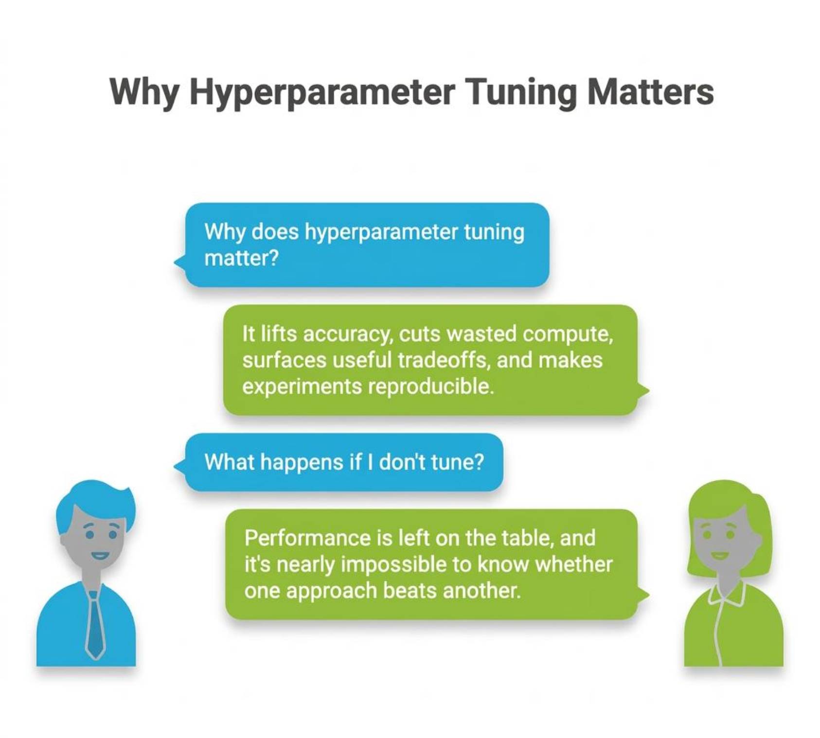
Hyperparameters are chosen by you. They control the training process rather than being learned from the data directly. Learning rate, batch size, number of epochs, tree depth, dropout, and regularization strength all fall into this category.
That difference matters because a model cannot fix a poor training setup on its own. A strong model with weak hyperparameters can still produce disappointing results.
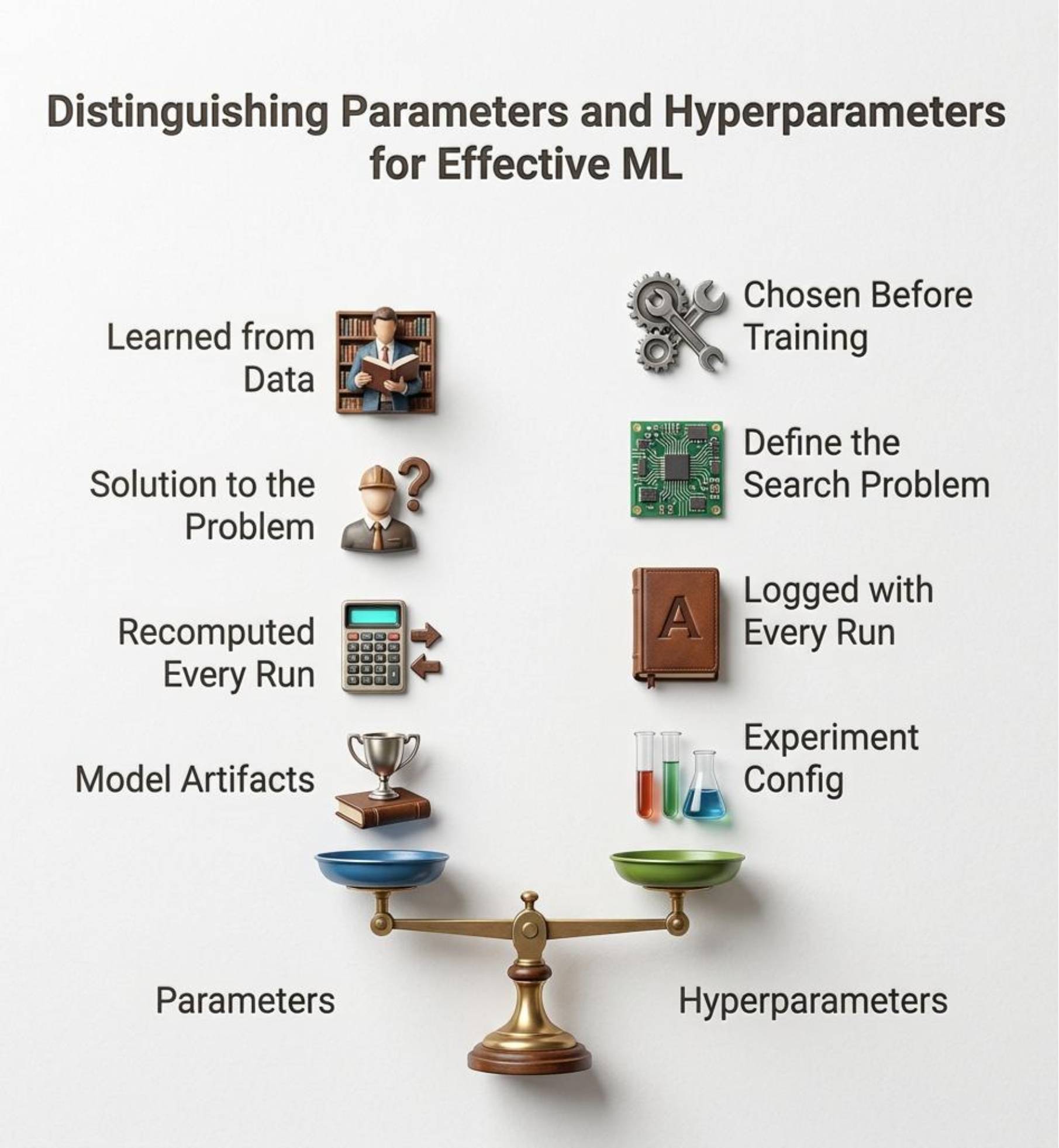
In practice, the point is simple. Parameters are what the model discovers. Hyperparameters are the conditions you create for that discovery.
There are three common approaches.
Grid search tries every combination in a predefined set. It is easy to understand and easy to explain, but it becomes expensive quickly.
Random search samples configurations from the ranges you define. In many real projects, this is the best default because only a small subset of hyperparameters matters a lot, and random search covers more useful ground than grid search with the same budget.
Bayesian optimization uses the results of earlier trials to decide what to try next. It is more adaptive and usually more sample-efficient, which makes it attractive when each run is slow or expensive.
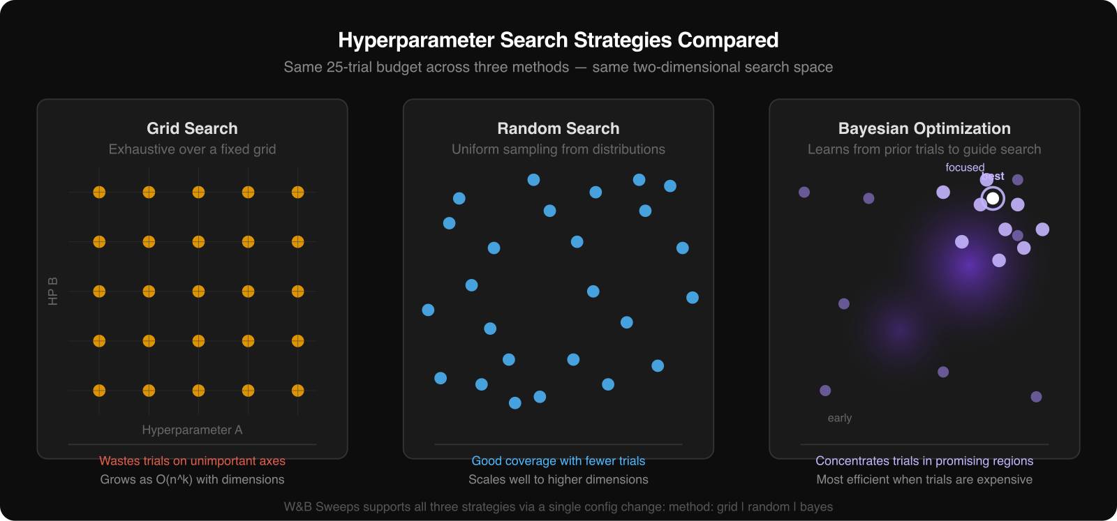
The right method depends on the cost of a run and the size of the search space. For a simple tutorial or a fast baseline model, random search is often enough. For expensive models, Bayesian methods become more attractive.
The most common mistake in hyperparameter tuning is using the test set too early.
When you compare configurations, you need three data splits:
If the test set influences your tuning decisions, even indirectly, the final score ceases to be honest. It becomes part of the search process.
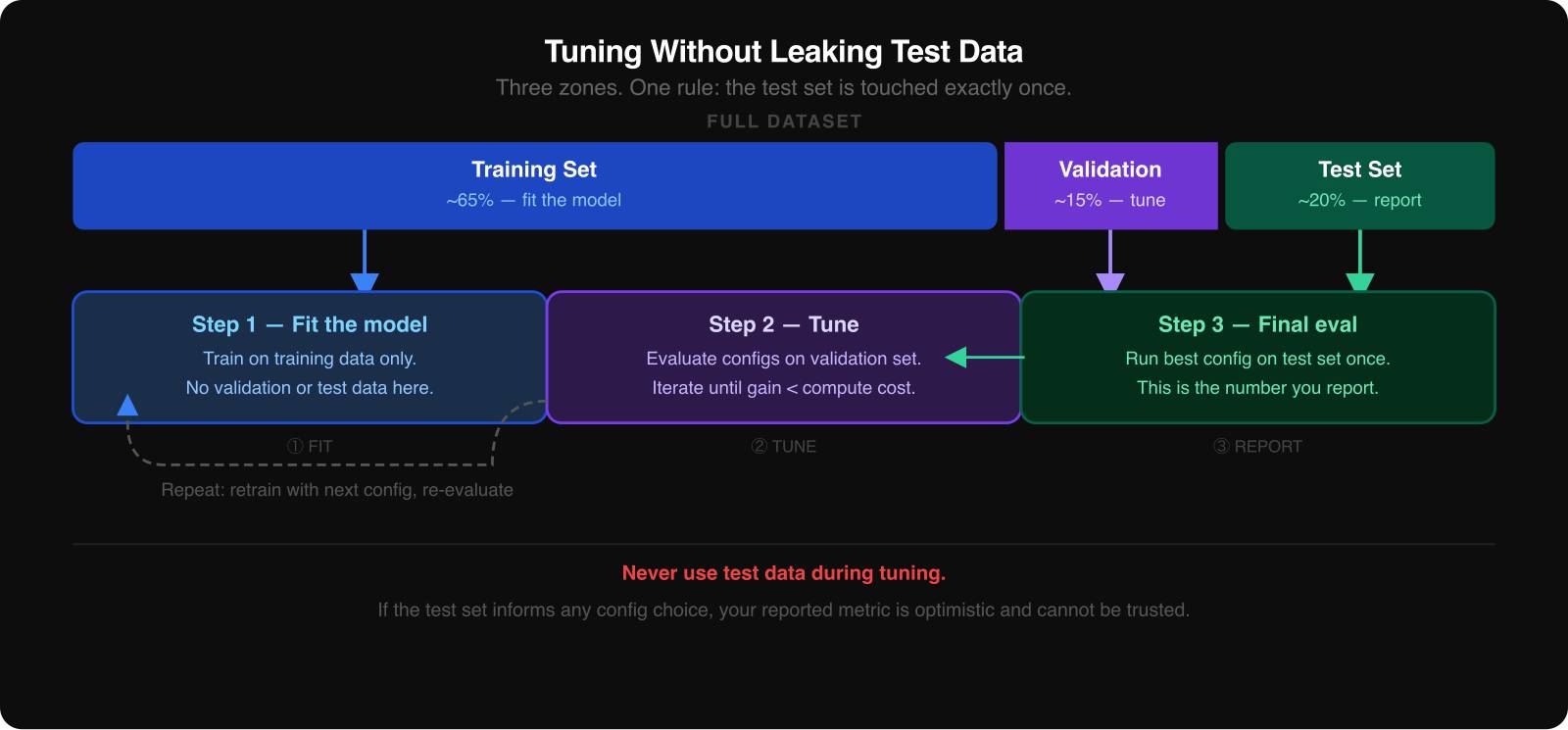
The safest way to think about the test set is as a sealed envelope. You open it once, after you have already chosen the winning configuration from the validation results.
There is one important exception in the experiment section of this article. The breast-cancer dataset is small, so the sweeps use 5-fold stratified cross-validation rather than a single held-out validation and test split. That means the reported scores later in the article are cross-validation AUC values, not a single, untouched test-set score. The principle is still the same: the evaluation protocol must stay fixed and must not leak information across runs.
Hyperparameter tuning becomes messy once you stop running just two or three experiments. You end up with screenshots, half-remembered settings, terminal logs, and filenames that no longer tell you what happened.
W&B solves that tracking problem first. Every run can log its configuration, metrics, summaries, and output artifacts in one place. Once that is in place, sweeps become much easier to reason about because you can compare runs side by side instead of reconstructing them from memory.
To show this in practice, this project uses two sweeps on the Wisconsin Breast Cancer Diagnostic dataset. The original dataset is hosted by UCI, and in the code, it is loaded through scikit-learn’s load_breast_cancer() helper. It has 569 rows, 30 numeric features, and a binary diagnosis target.
One sweep uses XGBoost. The other uses a neural network built with scikit-learn’s MLPClassifier. Both optimize 5-fold cross-validation AUC, use Bayesian search, and run 30 trials with Hyperband early termination.
You can inspect the live runs here:
The XGBoost sweep looks like this:
import wandb
from sklearn.datasets import load_breast_cancer
from sklearn.model_selection import StratifiedKFold, cross_val_score
from sklearn.preprocessing import StandardScaler
from xgboost import XGBClassifier


def train():
    with wandb.init() as run:
        cfg = run.config
        X, y = load_breast_cancer(return_X_y=True)
        X = StandardScaler().fit_transform(X)

        model = XGBClassifier(
            max_depth=cfg.max_depth,
            learning_rate=cfg.learning_rate,
            subsample=cfg.subsample,
            colsample_bytree=cfg.colsample_bytree,
            min_child_weight=cfg.min_child_weight,
            gamma=cfg.gamma,
            n_estimators=cfg.n_estimators,
            eval_metric="auc",
            verbosity=0,
            random_state=42,
        )

        cv = StratifiedKFold(n_splits=5, shuffle=True, random_state=42)
        scores = cross_val_score(model, X, y, cv=cv, scoring="roc_auc")
        wandb.log({"val_auc": float(scores.mean())})


SWEEP_CONFIG = {
    "method": "bayes",
    "metric": {"name": "val_auc", "goal": "maximize"},
    "parameters": {
        "max_depth": {"values": [3, 4, 5, 6, 7, 8]},
        "learning_rate": {"distribution": "log_uniform_values", "min": 0.01, "max": 0.3},
        "subsample": {"distribution": "uniform", "min": 0.5, "max": 1.0},
        "colsample_bytree": {"distribution": "uniform", "min": 0.5, "max": 1.0},
        "min_child_weight": {"values": [1, 3, 5, 7]},
        "gamma": {"distribution": "uniform", "min": 0.0, "max": 1.0},
        "n_estimators": {"values": [50, 100, 200, 300]},
    },
    "early_terminate": {"type": "hyperband", "min_iter": 5},
}

sweep_id = wandb.sweep(SWEEP_CONFIG, project="hyperparameter-tuning-article")
wandb.agent(sweep_id, function=train, count=30)
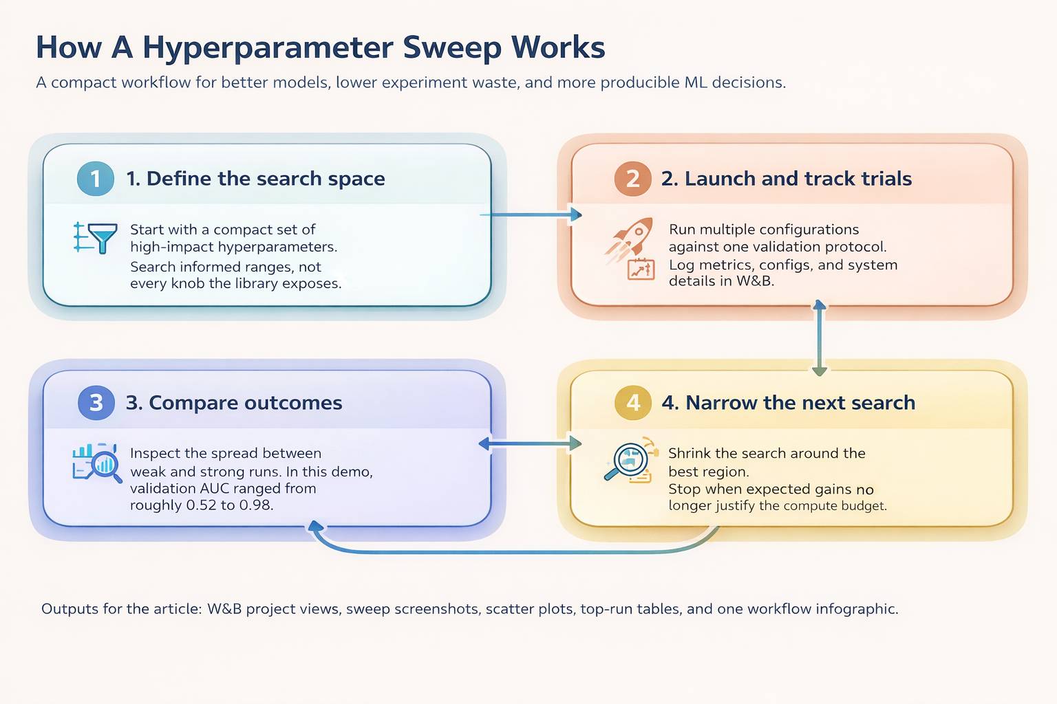
This is where W&B earns its keep. It lets you inspect the search instead of treating it like a black box. You can see which configurations improved the metric, which regions of the search space kept producing strong runs, and which parameters turned out not to matter much.
The experiment track used in the main article is built around the Wisconsin Breast Cancer Diagnostic dataset:
load_breast_cancer() in sweep_xgboost.py and sweep_neural_net.py56930 numeric inputsThis dataset works well for a tutorial because it is small enough to run quickly but structured enough to show real differences between hyperparameter choices.
The first sweep used XGBoost. The second used a neural network. Both used Bayesian optimization over 30 trials and scored each run with a mean 5-fold cross-validation AUC.
The goal was simple: run two different model families on the same dataset, tune both under the same evaluation protocol, and see which hyperparameters actually explained the performance differences.
The search spaces were:
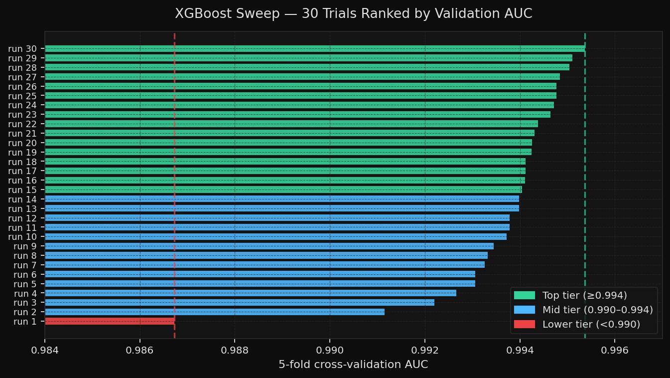
max_depth, learning_rate, subsample, colsample_bytree, min_child_weight, gamma, n_estimatorslearning_rate_init, hidden_layer_sizes, alpha, batch_size, activation, solverThe XGBoost results were strong and fairly stable. Validation AUC ranged from 0.9867 to 0.9954, indicating the model was already robust, and the sweep was mostly about closing the remaining gap.
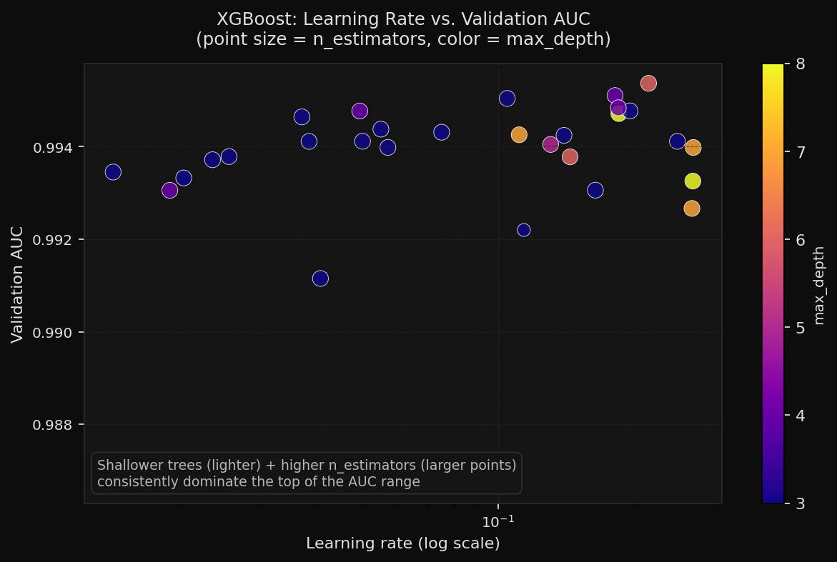
The learning-rate scatter makes the productive region easier to see. Across many trials, higher estimator counts and modest tree depth clustered near the top of the chart.
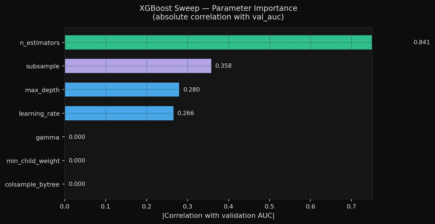
The parameter-importance view shows why the sweep converged quickly. In this run, n_estimators carried the strongest signal. Some other settings moved much less than expected, which means a follow-up sweep could safely be tighter.
The neural-network sweep told a noisier story. AUC ranged from 0.3622 to 0.9959 on the same dataset and the same evaluation objective. That spread is a good illustration of why tuning matters more for neural networks than for forgiving tabular models.
The neural network’s search space was also more interaction-heavy. It varied the learning rate, layer size, alpha, batch size, activation, and solver. Those choices do not act independently, which is why a neural network sweep often produces both excellent runs and very weak ones within the same budget.
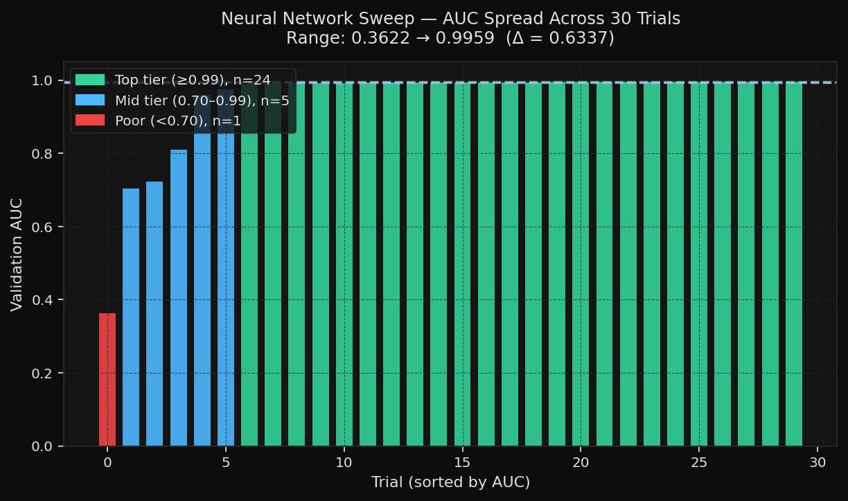
The parallel-coordinates view shows the interaction effect directly. The same activation and solver choices appeared in both strong and weak runs. Learning rate, regularization, and layer size were the factors that separated them.
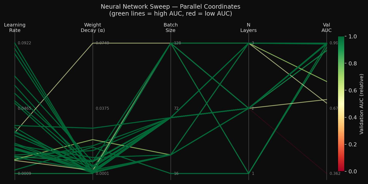
The best neural-network configuration was:
learning_rate_init = 0.0883hidden_layer_sizes = [64, 32]alpha = 0.00078batch_size = 16activation = logisticsolver = sgdThe best XGBoost run achieved an AUC of 0.9954. The best neural network achieved an AUC of 0.9959. The more important takeaway is not the tiny gap between the best scores. It is the shape of the search. XGBoost was comparatively stable across trials, while the neural network was much more sensitive to configuration. That is the kind of result a sweep is supposed to reveal.